KiCad is a great tool for taking your electronics design from schematic to PCB, but circuit simulation is secondary feature.
As we will see here KiCad does contain the ability to generate netlists which can be used with simulators like ngspice to perform circuit verification and analysis.
To get started we will need to decide on a design. I will choose a circuit which will show us how to do following:
- Use vendor spice components
- Perform Transient Analysis
- Simulate an input signal
- Measure frequency responce
Layout Circuit and Generate Netlist
For this demo let us pick a simple inverting op amp circuit. We can use the spice models from vendors like Texas Instruments and Linear Technology to provide the op amp. This also means we can easily, virtually, swap out components to see how they perform in our design.
Below we can see the completed schematic for a non-inverting op amp with a dual power supply. The 50K ohm feedback and 2K ohm input resistors mean our signal will be amplified 25 times. For more details on drawing schematics in kicad refer to the getting started tutorials.
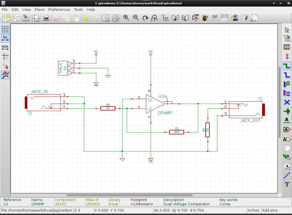
Image 1: The completed inverting op amp schematic
Once our circuit is complete we can generate a spice netlist by navigating to Tools > Generate Netlist.
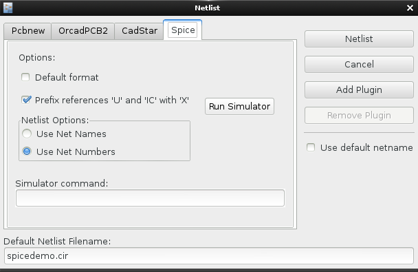
Image 2: Generating the spice netlist
Some comments on the Netlist options:
- The Default format option does not seem to do anything
- I have selected Prefix references ‘U’ and ‘IC’ with ‘X’, this is needed for
ngspiceas it recognizes ‘X’ components as subcircuits. However for the Jack and Power interfaces annotated withJ*andP*it would be nice to prefix with X as we will implement these with subcircuits as well.
Once the options are selected click Netlist to save your netlist. This will generate a netlist like the following:
* EESchema Netlist Version 1.1 (Spice format) creation date: Sat 25 Apr 2015 07:04:41 AM JST

* To exclude a component from the Spice Netlist add [Spice_Netlist_Enabled] user FIELD set to: N
* To reorder the component spice node sequence add [Spice_Node_Sequence] user FIELD and define sequence: 2,1,0

*Sheet Name:/
XU1  7 6 0 4 1 OPAMP
J1  2 0 0 JACK_IN
J2  7 3 0 JACK_OUT
R2  6 7 50K
R1  2 6 2K
R3  0 3 2K
P1  4 0 1 PWR_IN

.end
Setup Inputs and Outputs for Simulation
In order to simulate the circuit we need to plug in our virtual power supplies, signal generators and oscilloscope probes. To do this I have chosen to use subcircuits to contain each or these test components.
Create a components.cir like the following:
* Components and subcircuits for use in spicedemo.cir

.INCLUDE LMV981.MOD

* 4 0 1 PWR_IN
*              + g -
.subckt PWR_IN 1 2 3
  Vneg 1 2  3.3V
  Vpos 2 3 3.3V
.ends PWR_IN

* 7 6 0 4 1 OPAMP
*             o - + p n
.subckt OPAMP 1 2 3 4 5
  * PINOUT ORDER  1   3   6  2  4   5
  * PINOUT ORDER +IN -IN +V -V OUT NSD
  Xopamp 3 2 4 5 1 NSD LMV981
.ends OPAMP

*               s x g
.subckt JACK_IN 1 2 3
  *** Simulate mic input A-note
  Vmic  3 1 ac SIN(0 0.02 440)
.ends JACK_IN

*                s x g
.subckt JACK_OUT 1 2 3
  Rwire  1 2   10ohm
.ends JACK_OUT
PWR_IN : Connecting Power
This first subcircuit is the PWR_IN connector in our kicad circuit. This is a 3pin connector with a positive rail, negative rail and ground. Here we use two DC power supplies to generate the positive and negative rails. Be sure to double check pin numbers with your generated netlist.
OPAMP : The IC
Next we have the OPAMP subcircuit. For this we just provide a wrapper for the component included with .INCLUDE LMV981.MOD. This spice model from Texas Instruments and was selected as it provides a 6 pin low power solution. Many vendors provide models like this which can be used.
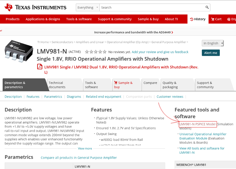
Image 3: Here we can see how to download spice models from Texas Instruments
JACK_IN : Simulating Microphone Input
The JACK_IN and JACK_OUT interfaces are typical mono audo jack interface with 3 pins (called jack 2-pole). The 3 pins are ‘signal’ (tip), ‘ground’ (sleeve) and ‘normally closed (NC)’. When the jack has nothing plugged into it the ‘signal’ and ‘normally closed’ pins will be shorted. When the jack has something plugged in (like a microphone) then the ‘signal’ and ‘ground’ pins will be connected to the microphone and ‘normally closed’ is disconnected. The reason for this is to protect from having floating inputs or outputs or use for jack plug-in detection.
Note: For details on jacks read the wiki and manufacturer documents from Schurter, Adam Tech and Farnell
For JACK_IN we simulate a microphone plugged in by providing a 440hz (a-note) sine wave of 20mV, a typical microphone signal.
JACK_OUT : Simulating a Load
For JACK_OUT we use the dummy load resistor R3 to provide some load to the op amp output. To wire together ‘signal’ and ‘unplugged’ pins we just add a dummy 10ohm resistor. It could have been 0 or 1 ohm, but I just set it to 10.
Update the Generated Netlist
Next, we need to go back and modify the generated netlist slightly to include the components.cir and perform the analysis we wish to do. Also, because we are using subcircuits we add X’s to the J and P components.
Note: Instead of manually adding .include and analysis lines we could add -PSPICE and +PSPICE text blocks anywhere to our kicad schematic and it will include the text before and after the netlist respectively.
.include components.cir

*Sheet Name:/
XU1  7 6 0 4 1 OPAMP
XJ1  2 0 0 JACK_IN
XJ2  7 3 0 JACK_OUT
R2  6 7 50K
R1  2 6 2K
R3  0 3 2K
XP1  4 0 1 PWR_IN

.op

.tran 0.1m 3m
.plot tran V(7) V(2)

.ac dec 10 1 100K
.plot ac V(7)

.end
Simulation
Running OP Analysis
First its always good to run the dc operating, OP, analsysis to make sure nothing is shorted.
Because we have included the op amp spice model the full analsysis results in more than a thousand lines for dc analysis. The main things to look at our our voltages and currents.
We can check the important voldages with grep as below. Here we can see relatively low voltages other than our supplies which looks normal.
$ ngspice -b spicedemo.cir | grep V\(

        V(3)                             -2.85334e-02
        V(2)                             0.000000e+00
        V(7)                             -2.86760e-02
        V(6)                             -1.13177e-03
        V(1)                             -3.30000e+00
        V(4)                             3.300000e+00
To view the currents we can run a similar grep and see similar low values (less than 1 milliamp). Its good to look at the entire output to understand how these greps work.
$ ngspice -b spicedemo.cir | grep v\\.x

        v.xj1.vmic#branch                5.658851e-07
        v.xp1.vneg#branch                -1.37178e-04
        v.xp1.vpos#branch                -1.51996e-04
Running TRAN Analysis.
Next we can run the TRAN analsysis (oscilloscope mode), to make sure it works. Here we can see that the input signal is amplified from 20mV to 500mV resulting in our expected 25 times gain. The result is also inverted as we are using an inverting amp configuration.
# In interactive mode
$ ngspice spicedemo.cir

> tran 0.3m 1m
> plot V(2) V(7)
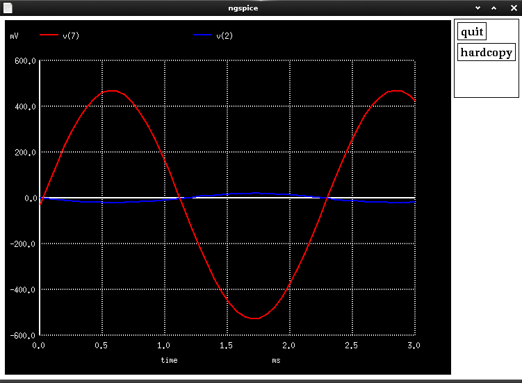
Image 4: Transient analysis, shows the input signal in blue and output in red
Running AC Analysis
Finally running AC analysis we can measure the frequency responce (bandwidth) of the circuit. Below we can see that after about 10,000 Hz the gain starts to drop off.
# In interactive mode
$ ngspice spicedemo.cir

> ac dec 10 1 100K
No. of Data Rows : 51
> plot V(2) V(7)
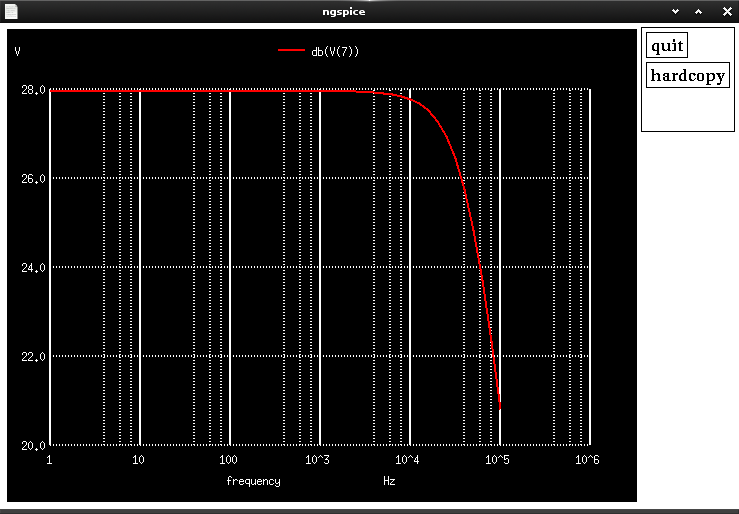
Image 5: Shows performance drop off after 10K hz
Further Reading
- Mathat Konar Quick Guide Short guide explains using libraries and
+PSPICE-PSPICE